Chapter 19 Knowledge graphs and IRT
Learning goals. After this chapter you can
- describe what a test measures as a knowledge graph of concepts,
prerequisites and items, and build one with
mv_kg_build()oras_mv_kg(); - check a graph for problems with
mv_kg_check()and draw it withgg_kg(); - read a graph’s Q-matrix and list the mastery patterns its attribute hierarchy allows;
- turn a graph into a confirmatory multidimensional IRT model with
mv_kg_model()andmv_kg_irt(), and test the graph’s claims against simpler and stricter models; - check a graph against data with
mv_kg_fit()and explain item difficulty with it usingmv_kg_explain(), with item metadata as extra predictors; - draft a graph from item text with a language model using
mv_kg_extract(), and review the draft against an expert graph withmv_kg_compare().
Key terms: Knowledge graph, Q-matrix, attribute hierarchy, multidimensional IRT, likelihood-ratio test.
19.1 The ideas
Every test is built on claims about what it measures. A blueprint says which content each item covers; a curriculum says that some ideas must be learned before others; a teacher knows that an item about subtracting mixed numbers also needs borrowing. Most of these claims stay in documents and heads. A knowledge graph writes them down in a form a computer can check and a model can use. It has three kinds of parts.
- Concepts (also called skills, attributes or objectives): What the test is meant to tell us about.
- Relations between concepts. The most useful is prerequisite of: Equivalent fractions before adding fractions with unlike denominators. Prerequisite edges point forward in the learning order and should never form a cycle. A weaker relation, related to, links concepts where neither comes first.
- Items, each linked to the concepts it measures. These links are the rows of the Q-matrix (Tatsuoka 1984): One row per item, one column per concept, with a 1 where the item needs the concept.
The graph connects two traditions in psychometrics. In multidimensional IRT, the Q-matrix is the loading pattern of a confirmatory model: Each concept is a factor, and an item has a slope only on the concepts it measures (Chapter 4). In cognitive diagnosis, the same Q-matrix says which skills an item needs, and prerequisite edges form an attribute hierarchy (Leighton et al. 2004; Templin and Bradshaw 2014): A student can master a concept only after mastering its prerequisites, so some mastery patterns are impossible. Knowledge space theory (Doignon and Falmagne 1999) builds a whole theory of assessment on such structures.
A graph is a set of claims, and each claim can be wrong. An item can be linked to the wrong concept, a prerequisite can be missing or reversed, and two concepts can be impossible to tell apart because the same items measure them. The work in this chapter is to make the claims explicit, check what can be checked without data, and then let the data speak.
19.2 Example 1: A graph for fraction subtraction
Tatsuoka’s fraction subtraction data are the best-known real data in
cognitive diagnosis: 536 middle school students answered 20 items such as
\(4\frac{1}{3} - 2\frac{4}{3}\), and the items were coded on eight
attributes (Tatsuoka 2002; DeCarlo 2011; Torre and Douglas 2004). mirtverse
stores the responses as fraction_subtraction and the Q-matrix as a
knowledge graph, fraction_subtraction_kg.
kg
#> <mv_kg> Fraction subtraction (Tatsuoka): 8 concept(s), 20 item(s)
#> Edges: 0 prerequisite, 0 related, 56 measures
#> Item metadata: text
tidy(kg)
#> # A tibble: 28 × 6
#>   node               kind    label                       description links depth
#>   <chr>              <chr>   <chr>                       <chr>       <dbl> <dbl>
#> 1 convert_whole      concept Convert a whole number to … Attribute …     3     0
#> 2 separate_whole     concept Separate a whole number fr… Attribute …    13     0
#> 3 simplify_first     concept Simplify before subtracting Attribute …     3     0
#> 4 common_denominator concept Find a common denominator   Attribute …     5     0
#> 5 borrow_whole       concept Borrow from the whole numb… Attribute …     8     0
#> 6 column_borrow      concept Column borrow to subtract … Attribute …     2     0
#> # ℹ 22 more rows
The graph has eight concepts and 20 items, with 56 item-to-concept links.
No prerequisite edges were published with the Q-matrix, so the graph has
none yet. tidy() counts the items linked to each concept (links).
subtract_numerators is needed by 19 of the 20 items, while
column_borrow is needed by only two. Before any data are used,
mv_kg_check() looks for problems in the structure itself.
mv_kg_check(kg)
#> <mv_kg_check> 0 block, 1 review, 0 info
#> * [review] few_items: column_borrow is measured by 2 item(s); at least
#>   3 are needed to estimate it as its own dimension.
The check finds one thing to review: Two items are too few to estimate
column_borrow as its own dimension. A concept that nearly every item
needs, like subtract_numerators, has the opposite problem: It is hard to
separate from overall proficiency. Neither is an error in the graph, but
both limit what a model can learn about these concepts.
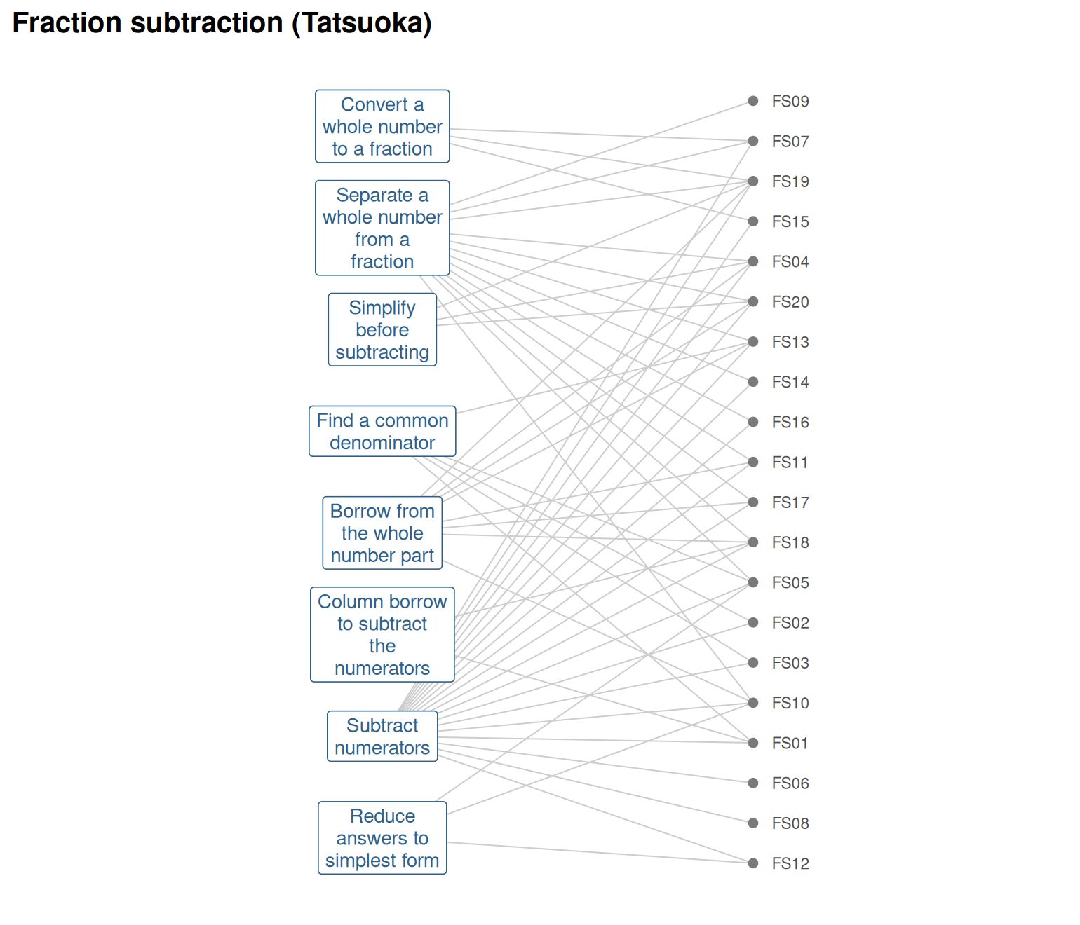
Figure 19.1: The fraction subtraction graph: Eight attributes on the left, each joined to the items that need it.
Now suppose a mathematics teacher states two prerequisites as hypotheses: Borrowing from the whole number needs the whole number to be separated from the fraction first, and column borrowing needs subtracting numerators. We add these edges to the same concepts and items.
concepts <- tidy(kg)
concepts <- concepts[concepts$kind == "concept", ]
kg_h <- mv_kg_build(
  concepts = data.frame(concept = concepts$node, label = concepts$label),
  edges = data.frame(from = c("separate_whole", "subtract_numerators"),
                     to = c("borrow_whole", "column_borrow")),
  items = mv_kg_qmatrix(kg),
  name = "Fraction subtraction with two prerequisites")
kg_h
#> <mv_kg> Fraction subtraction with two prerequisites: 8 concept(s), 20 item(s)
#> Edges: 2 prerequisite, 0 related, 56 measures
#> Learning order (by prerequisite depth):
#>   0: convert_whole, separate_whole, simplify_first, common_denominator, subtract_numerators, reduce_answer
#>   1: borrow_whole, column_borrow
The print-out now gives a learning order. The hierarchy has a practical consequence: With eight concepts there are \(2^8 = 256\) possible mastery patterns, and each prerequisite rules out the patterns where a concept is mastered without its prerequisite.
Two edges remove 112 of the 256 patterns. A diagnostic model that respects the hierarchy has fewer classes to estimate, and the hierarchy itself can be tested by comparing models with and without it.
19.3 Example 2: From graph to IRT model
mv_kg_model() writes the confirmatory mirt model a graph implies, and
mv_kg_irt() fits it. Eight correlated dimensions on 536 students is a
large model that takes many minutes to fit, so we work with a smaller
graph: The three concepts with the clearest roles, separating the whole
number, borrowing, and finding a common denominator. mv_kg_subset() keeps
these concepts, the prerequisite between two of them, and the 16 items that
need at least one of them.
kg3 <- mv_kg_subset(kg_h, c("separate_whole", "borrow_whole", "common_denominator"))
kg3
#> <mv_kg> Fraction subtraction with two prerequisites: 3 concept(s), 16 item(s)
#> Edges: 1 prerequisite, 0 related, 26 measures
#> Learning order (by prerequisite depth):
#>   0: separate_whole, common_denominator
#>   1: borrow_whole
q <- mv_kg_qmatrix(kg3)
resp3 <- resp[rownames(q)]
spec <- mv_kg_model(kg3)
cat(attr(spec, "item_syntax"))
#> separate_whole = FS04, FS05, FS07, FS09, FS10, FS11, FS13, FS14, FS16, FS17, FS18, FS19, FS20
#> common_denominator = FS01, FS02, FS03, FS05, FS13
#> borrow_whole = FS04, FS10, FS11, FS13, FS17, FS18, FS19, FS20
#> COV = separate_whole*common_denominator, separate_whole*borrow_whole, common_denominator*borrow_whole
Each concept is a factor, and each item loads on the concepts its row of
the Q-matrix names; items that need two concepts load on both. By default
all concepts correlate. The structure argument changes that:
structure = "graph" lets only concepts joined by an edge correlate, a
strict reading of the graph in which concepts without an edge are
unrelated.
m_uni <- mirt(resp3, 1, verbose = FALSE)
m_graph <- mv_kg_irt(kg3, resp3)
m_strict <- mv_kg_irt(kg3, resp3, structure = "graph")
anova(m_uni, m_graph)
#>          AIC SABIC   HQ  BIC logLik     X2 df p
#> m_uni   7739  7775 7793 7876  -3838
#> m_graph 7371  7421 7447 7564  -3641 394.06 13 0
anova(m_strict, m_graph)
#>           AIC SABIC   HQ  BIC logLik      X2 df p
#> m_strict 7641  7689 7713 7825  -3778
#> m_graph  7371  7421 7447 7564  -3641 273.834  2 0
Two comparisons answer two questions. Against a single dimension, the three-concept model fits far better: The likelihood-ratio statistic is about 394 on 13 degrees of freedom, and BIC drops by more than 300. The items measure more than one proficiency, in the way the graph describes. Against the strict model, the correlated model also wins clearly: Finding a common denominator has no edge in the graph, yet it correlates with the other two concepts.
round(summary(m_graph, verbose = FALSE)$fcor, 2)
#>                    separate_whole common_denominator borrow_whole
#> separate_whole               1.00               0.77         0.38
#> common_denominator           0.77               1.00         0.39
#> borrow_whole                 0.38               0.39         1.00
Separating the whole number and finding a common denominator correlate at about 0.77, much more than the two concepts the teacher linked (about 0.37). This is a typical finding, not a failure: A prerequisite edge says something about the order of learning, and concepts that are learned in the same lessons correlate whether or not one is a prerequisite of the other. The correlations are a reason to look again at the graph, for example to ask whether a related-to edge is missing.
The fitted model is an ordinary mirt model, so everything from the earlier chapters works on it, and the graph travels with it.
pars <- tidy(m_graph)
head(pars[pars$estimate != 0, ])
#> # A tibble: 6 × 5
#>   item  itemtype term  estimate std.error
#>   <chr> <chr>    <chr>    <dbl>     <dbl>
#> 1 FS01  2PL      a2       5.13         NA
#> 2 FS01  2PL      d        1.08         NA
#> 3 FS02  2PL      a2       7.39         NA
#> 4 FS02  2PL      d        2.31         NA
#> 5 FS03  2PL      a2      13.8          NA
#> 6 FS03  2PL      d        0.943        NA
attr(m_graph, "mv_kg")
#> <mv_kg> Fraction subtraction with two prerequisites: 3 concept(s), 16 item(s)
#> Edges: 1 prerequisite, 0 related, 26 measures
#> Learning order (by prerequisite depth):
#>   0: separate_whole, common_denominator
#>   1: borrow_whole
as_mv_kg() also goes the other way: Given any confirmatory mirt model, it
reads the loading pattern back into a graph, which is a quick way to draw a
model you already have.
19.4 Example 3: Checking the graph against data
The comparisons above test the graph as a whole. mv_kg_fit() looks for
the places where the data disagree with it. For each item, it asks whether
the item agrees more with another concept than with its own: It correlates
the item with the rest score of every concept, corrected for how reliable
each rest score is. For each pair of concepts, it turns the factor
correlations of the correlated model into partial correlations, the
correlation of two concepts once the others are held constant. Concepts
that are directly related keep a clear partial correlation; concepts
related only through others do not. We can pass in the model we already
have.
check <- mv_kg_fit(kg3, resp3, model = m_graph)
check
#> <mv_kg_fit> Fraction subtraction with two prerequisites: 3 concept(s), 16 item(s), N = 536
#> 2 review, 0 info
#> * [review] weak_link: FS13 is linked to separate_whole,
#>   common_denominator, borrow_whole but agrees much less with
#>   common_denominator than with separate_whole (r = 0.57 vs 0.70); drop
#>   the link to common_denominator?
#> * [review] missing_relation: separate_whole and common_denominator have
#>   no edge but a partial correlation of 0.73, and their items are about
#>   equally hard; add a related edge?
#> Item links shape the concept correlations: Fix item flags first and
#> refit before acting on relation flags.
tidy(check, "relations")
#> # A tibble: 3 × 10
#>   concept_a        concept_b edge  from  to    type      r partial ease_a ease_b
#>   <chr>            <chr>     <chr> <chr> <chr> <chr> <dbl>   <dbl>  <dbl>  <dbl>
#> 1 separate_whole   common_d… none  <NA>  <NA>  <NA>  0.771   0.731  0.487  0.500
#> 2 separate_whole   borrow_w… sepa… sepa… borr… prer… 0.382   0.137  0.487  0.410
#> 3 common_denomina… borrow_w… none  <NA>  <NA>  <NA>  0.391   0.164  0.500  0.410
Every item agrees best with a concept it is linked to, so there is no
wrong_link flag. One item gets a weak_link flag instead: FS13
(3 3/8 - 2 5/6) is linked to three concepts but agrees much less with
finding a common denominator than with separating the whole number. Look
at the item before acting on that: Eighths and sixths do need a common
denominator, so the link is right on content. Nearly every item with a
whole number part also needs separating and borrowing, which share most
of their items, so those concepts’ rest scores track FS13 more closely.
This is a flag to reject, and a reminder that the checks are screening
heuristics.
The relation evidence makes the earlier observation precise. Holding borrowing constant, separating the whole number and finding a common denominator still have a partial correlation of about 0.73, while the teacher’s prerequisite (separate_whole -> borrow_whole) drops to about 0.14. Because the two concepts’ items are about equally hard, the suggestion is a related edge rather than a prerequisite.
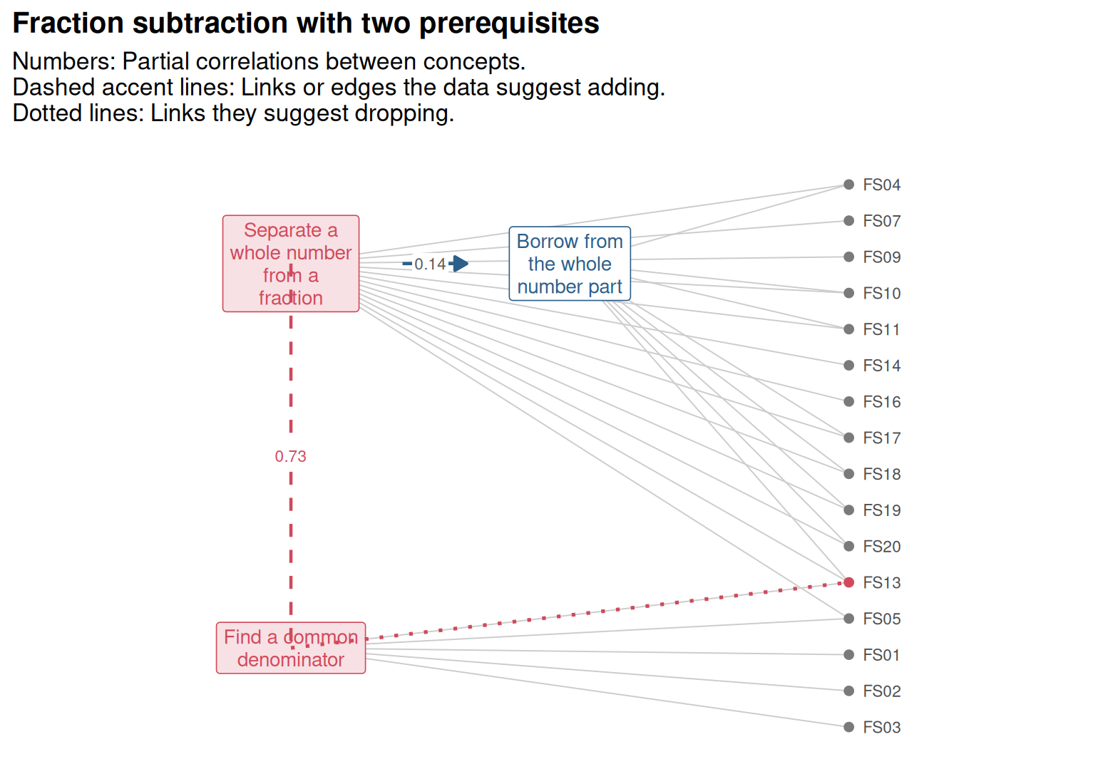
Figure 19.2: The evidence on the three-concept graph: Partial correlations next to each pair, the suggested related edge as a dashed line, and the weak link of FS13 as a dotted line.
mv_kg_refine(check, "relations") would add the edge and leave the
item links alone. Whether to do so is a content
question: Both skills come up when students handle mixed numbers with
unlike denominators, so a related edge is plausible, but the data alone
cannot say why the concepts go together.
A graph also makes claims about difficulty. mv_kg_explain() fits an
explanatory Rasch model with the eirm package (Bulut et al. 2021) in which
the graph predicts each item’s difficulty: One difficulty per concept (a
linear logistic test model, with a random item effect for what the
concepts leave unexplained), or the item’s depth in the learning order.
explain <- mv_kg_explain(kg, resp)
explain
#> <mv_kg_explain> Fraction subtraction (Tatsuoka): Item difficulty explained by concepts
#> 20 items, N = 536. The graph explains 88% of the item variance.
#>                label difficulty   se p.value
#>        convert_whole       2.10 0.29  <0.001
#>       separate_whole      -0.18 0.23    0.42
#>       simplify_first      -0.40 0.33    0.22
#>   common_denominator       1.32 0.24  <0.001
#>         borrow_whole       2.33 0.29  <0.001
#>        column_borrow      -0.01 0.33    0.98
#>  subtract_numerators      -1.69 0.22  <0.001
#>        reduce_answer       0.11 0.28    0.70
#> Items the graph predicts poorly: FS09 (-0.91).
The eight attributes explain most of the differences in item difficulty. Borrowing from the whole number and converting a whole number to a fraction add the most difficulty, and subtracting numerators, which almost every item needs, the least. The teacher’s two prerequisites, in contrast, say little about difficulty:
mv_kg_explain(kg_h, resp, predictors = "depth")
#> <mv_kg_explain> Fraction subtraction with two prerequisites: Item difficulty explained by learning-order depth
#> 20 items, N = 536. The graph explains 64% of the item variance.
#>                 label difficulty   se p.value
#>  Learning-order depth       0.47 0.49  0.3354
#>    Number of concepts       0.63 0.21  0.0024
Items that need more attributes are harder, but once that is taken into account, an item’s depth in the teacher’s learning order adds little. A prerequisite that does not show up as a difference in difficulty is not necessarily wrong, but it is a claim the data do not support yet.
Other things known about the items can join the concepts. A graph carries
item metadata: fraction_subtraction_kg has the text of each problem,
and mv_kg_annotate() adds more columns. Teachers often say that larger
denominators make a problem harder. Take the largest denominator in each
problem from its text and add it to the model:
denominator <- vapply(regmatches(kg$meta$text, gregexpr("/[0-9]+", kg$meta$text)),
                      function(d) max(as.numeric(sub("/", "", d))), numeric(1))
kg_m <- mv_kg_annotate(kg, data.frame(item = kg$meta$item, denominator = denominator))
tidy(kg_m, "items")[1:5, ]
#> # A tibble: 5 × 5
#>   item  concepts                                    n_concepts text  denominator
#>   <chr> <chr>                                            <int> <chr>       <dbl>
#> 1 FS01  common_denominator, column_borrow, subtrac…          3 5/3 …           4
#> 2 FS02  common_denominator, subtract_numerators              2 3/4 …           8
#> 3 FS03  common_denominator, subtract_numerators              2 5/6 …           9
#> 4 FS04  separate_whole, simplify_first, borrow_who…          4 3 1/…           2
#> 5 FS05  separate_whole, common_denominator, subtra…          4 4 3/…          10
mv_kg_explain(kg_m, resp, covariates = "denominator")
#> <mv_kg_explain> Fraction subtraction (Tatsuoka): Item difficulty explained by concepts and item metadata
#> 20 items, N = 536. The graph explains 88% of the item variance.
#>                label difficulty   se p.value
#>        convert_whole       2.09 0.30  <0.001
#>       separate_whole      -0.17 0.24    0.47
#>       simplify_first      -0.44 0.38    0.24
#>   common_denominator       1.34 0.26  <0.001
#>         borrow_whole       2.34 0.29  <0.001
#>        column_borrow       0.00 0.34    1.00
#>  subtract_numerators      -1.70 0.24  <0.001
#>        reduce_answer       0.15 0.35    0.66
#>          denominator      -0.01 0.05    0.83
#> Items the graph predicts poorly: FS09 (-0.90).
Once the attributes are in the model, the size of the denominator adds nothing: Its effect is close to zero and the share of item variance explained stays at 88%. What makes these items hard is the steps they need, not the numbers in them. The same check works for any item feature, such as word count, format, or whether a person or a language model wrote the item.
19.5 Example 4: Drafting a graph from item text
Writing a Q-matrix is slow, expert work: Someone has to read every item
and decide which skills it needs. A language model can read items too, so
it can draft the graph, and the expert’s job becomes reviewing the draft.
mv_kg_extract() sends the item text to a model (Chapter 17)
and asks for the item links and the prerequisites between concepts. Give
it the concepts, as here, and it only links items to them; leave them out
and it proposes the concepts too. The function is experimental.
We run it from the example recordings that come with mirtverse, so no
model or API key is needed. Those responses were written by the package
authors, with mistakes planted for the checks to catch; they are not the
output of a live model. With mv_ask_setup() the same call goes to Claude,
an OpenAI model or a local model.
old <- mv_llm_replay()
draft <- mv_kg_extract(kg, subject = "Middle school fraction subtraction")
draft
#> <mv_kg_draft> (EXPERIMENTAL) Drafted by recorded responses from the concepts given
#> <mv_kg> Fraction subtraction (Tatsuoka) (drafted): 8 concept(s), 20 item(s)
#> Edges: 7 prerequisite, 0 related, 54 measures
#> Item metadata: text
#> Learning order (by prerequisite depth):
#>   0: convert_whole, separate_whole, simplify_first, subtract_numerators
#>   1: common_denominator, borrow_whole, reduce_answer
#>   2: column_borrow
#> Checks on the model's answer: 5 flag(s)
#> * [review] unknown_item: The model linked FS21, which is not one of the
#>   items; the link was dropped.
#> * [review] unknown_concept: FS13 was linked to find_common_denominator,
#>   which is not a concept; the link was dropped.
#> * [review] two_way: The model gave the prerequisite both ways between
#>   simplify_first and reduce_answer; simplify_first -> reduce_answer was
#>   kept (higher confidence).
#> * [review] cycle: The prerequisites formed a cycle through
#>   subtract_numerators, borrow_whole, column_borrow; column_borrow ->
#>   subtract_numerators (confidence 0.3) was removed.
#> * [info] new_concept: The model proposed a new concept,
#>   subtract_whole_numbers; it was left out because the concepts were
#>   given.
#> Review the draft with mv_kg_check() and check it against data with mv_kg_fit().
Before the graph is built, the model’s answer is checked. Some problems
are simply errors and are fixed on the spot: A link to an item FS21 that
does not exist, and a concept the model was told not to add. Others are
fixed in a stated way: Where the model gave a prerequisite both ways, the
direction with higher confidence is kept, and the edge that closed a cycle
(the one with the lowest confidence) is removed. One fix costs
information: FS13 was linked to find_common_denominator, a misspelling,
so that link was dropped. Every model link comes with a reason:
reasons <- tidy(draft, "reasons")
reasons[reasons$from %in% c("FS04", "FS08"), c("from", "to", "reason")]
#> # A tibble: 5 × 3
#>   from  to                  reason
#>   <chr> <chr>               <chr>
#> 1 FS04  separate_whole      Work with the whole numbers and fractions separatel…
#> 2 FS04  simplify_first      3/2 is improper and can be simplified to 1 1/2 firs…
#> 3 FS04  subtract_numerators Subtract the fractional parts.
#> 4 FS08  subtract_numerators Like denominators; subtract the numerators.
#> 5 FS08  reduce_answer       The answer 0/3 should be written as 0.
Now compare the draft with the expert Q-matrix:
mv_kg_compare(draft, kg)
#> <mv_kg_compare> Fraction subtraction (Tatsuoka) (drafted) vs Fraction subtraction (Tatsuoka)
#> Item links: 53 of the 56 reference links are in the graph (recall
#>   0.95), and 53 of the graph's 54 links are in the reference (precision
#>   0.98).
#> 16 of 20 items are linked to exactly the same concepts.
#> Items that differ: FS01 (missing column_borrow), FS04 (missing
#>   borrow_whole), FS08 (extra reduce_answer), FS13 (missing
#>   common_denominator).
#> Prerequisites: The graph has 7; the reference has none to compare with.
options(old)
The model and the expert agree on 16 of the 20 items, and on 53 of the 56 expert links. The four differences are the places to look, and they are not all the model’s mistakes:
- FS13 is the misspelled link. The checks caught it, and the expert is right: Eighths and sixths need a common denominator.
- FS01 (5/3 - 3/4): The expert codes column borrowing and the model does not. This attribute is the hardest to apply from the text alone, and the coding is the expert’s call.
- FS04 (3 1/2 - 2 3/2): The model leaves out borrowing. Its reason is that 2 3/2 can be simplified to 3 1/2 first, after which there is nothing to borrow; the expert codes the usual procedure, which borrows. Both readings are defensible, and they describe different solution strategies.
- FS08 (2/3 - 2/3): The model adds reducing the answer, because 0/3 has to be written as 0. Again defensible, and a question for the item writers: Is that step part of what the item is meant to measure?
The draft’s prerequisites have nothing to compare with, because none were
published with the Q-matrix. They are hypotheses, and Example 3 showed how
to check such claims with data: Partial correlations with mv_kg_fit()
and depth with mv_kg_explain().
The lesson is the one that runs through this part of the book: A model’s output is a draft to be checked. Here three kinds of checks work together. The answer checks catch errors in what the model returned, the comparison with an expert graph shows where two readings of the items differ, and the data (Example 3) say which links and edges the students’ answers support. A draft that agrees with the expert on most items, with its disagreements listed, is a useful second opinion; it is not a replacement for the expert.
19.6 Your turn
- Add a third hypothesis to
kg_h: Converting a whole number to a fraction (convert_whole) is a prerequisite of borrowing (borrow_whole). How many mastery patterns are left? - Add a cycle by also making
borrow_wholea prerequisite ofseparate_whole. What doesmv_kg_check()report, and what happens tomv_kg_hierarchy()? - Fit the three-concept model with
structure = "orthogonal". How does it compare with the correlated model, and what does that say about scoring the three concepts separately? - Draw
kg3withgg_kg(), highlightingcommon_denominator. Which items does it share withseparate_whole?
Solutions
# 1. a third prerequisite
edges3 <- data.frame(from = c("separate_whole", "subtract_numerators", "convert_whole"),
                     to = c("borrow_whole", "column_borrow", "borrow_whole"))
kg_h3 <- mv_kg_build(data.frame(concept = concepts$node, label = concepts$label),
                     edges = edges3, items = mv_kg_qmatrix(kg))
nrow(mv_kg_hierarchy(kg_h3))
#> [1] 120

# 2. a cycle
kg_cyc <- mv_kg_build(data.frame(concept = concepts$node),
                      edges = rbind(edges3, data.frame(from = "borrow_whole",
                                                       to = "separate_whole")),
                      items = mv_kg_qmatrix(kg))
mv_kg_check(kg_cyc)
#> <mv_kg_check> 1 block, 1 review, 3 info
#> * [block] cycle: Prerequisite edges form a cycle through
#>   separate_whole, borrow_whole, so no learning order exists.
#> * [review] few_items: column_borrow is measured by 2 item(s); at least
#>   3 are needed to estimate it as its own dimension.
#> * [info] isolated: simplify_first has no relations to other concepts.
#> * [info] isolated: common_denominator has no relations to other
#>   concepts.
#> * [info] isolated: reduce_answer has no relations to other concepts.
try(mv_kg_hierarchy(kg_cyc))
#> Error : The prerequisite edges contain a cycle; see mv_kg_check().

# 3. uncorrelated concepts
m_orth <- mv_kg_irt(kg3, resp3, structure = "orthogonal")
anova(m_orth, m_graph)
#>          AIC SABIC   HQ  BIC logLik      X2 df p
#> m_orth  7642  7689 7712 7822  -3779
#> m_graph 7371  7421 7447 7564  -3641 276.773  3 0

# 4. shared items
gg_kg(kg3, highlight = "common_denominator")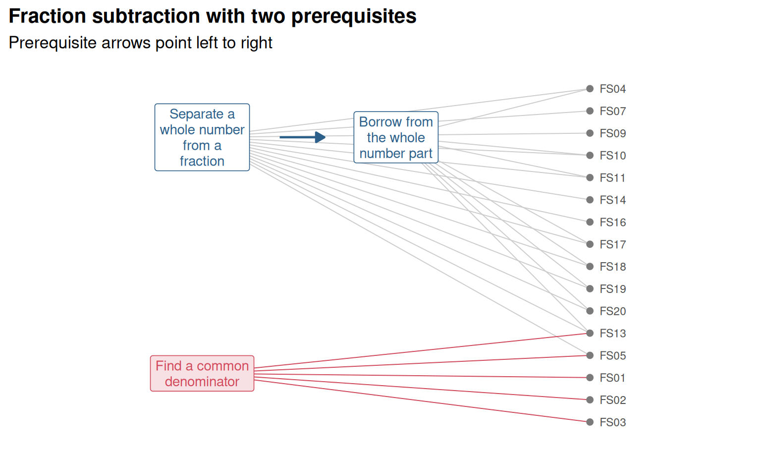
q[q[, "common_denominator"] == 1 & q[, "separate_whole"] == 1, ]
#>      separate_whole common_denominator borrow_whole
#> FS05              1                  1            0
#> FS13 1 1 1- Borrowing now needs both separating and converting, so more patterns are ruled out: 120 of the 256 remain.
- The check reports a
cycleblock flag: Separating the whole number would have to come both before and after borrowing, so no learning order exists.mv_kg_hierarchy()stops with an error, because a cycle allows no consistent set of patterns. - The orthogonal model fits much worse than the correlated one (the likelihood-ratio statistic is about 277 on 3 degrees of freedom). The concepts share a lot of variance, so three separate scores would repeat much of the same information; reporting them separately needs care (Chapter 12).
- Two items, FS05 and FS13, need both concepts; FS13 also needs borrowing. The other common denominator items (FS01 to FS03) involve no whole numbers. Items that load on two concepts help the model separate the concepts from their correlation.
In the lab
Lab 11, Repairing a knowledge graph (run_lab("kg-repair")): A
district’s curriculum team has written a knowledge graph for its Grade 5
fractions test, and diagnostic reports will follow it. Check the graph
against the students’ answers with mv_kg_fit(), find an item linked to
the wrong concept and a missing prerequisite, repair the graph with
mv_kg_refine(), and show what the repair changes.
Lab 12, Reviewing an AI-drafted graph (run_lab("kg-draft")): The
same district asks a language model to draft the graph from the item
text. Review the draft: Read the checks on the model’s answer, compare it
with the curriculum team’s graph, test both against the students’
answers, and decide what to keep.
Further reading
Tatsuoka (1984) introduced the Q-matrix with the fraction subtraction data; DeCarlo (2011) and de la Torre and Douglas (2004) reanalysed them with diagnostic models. Leighton, Gierl and Hunka (2004) describe the attribute hierarchy method, and Templin and Bradshaw (2014) show how to test hierarchies with diagnostic classification models. Doignon and Falmagne (1999) develop knowledge space theory, the mathematical theory of prerequisite structures in assessment.